What is the Geographic Buffer?#
Note
This tutorial requires basic GIS (Geographic Information System) knowledge.
What is the Buffer?#
Note
All buffer of geometries are created on 2D plane.
A simple graph could show this.

The graph shows the buffer generation of three basic kinds of geometries.
Point
Line
Polygon
And the graph also shows the way to deal with the overlapping relationship of multi-buffers.
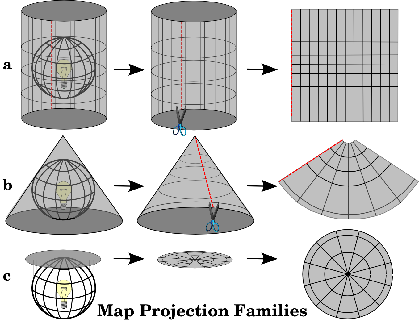
Latitude, Longitude and Earth#
This section comes to introduce CRS (Coordinate Reference Systems).
Simply say CRS shows a mapping relationship between 3D ellipsoid Earth and 2D plane.
Some CRSs we have already met, the GPS coordniate references, used in online map:
EPSG:4326: \((120°, 50°)\), spherical referenceEPSG:3857: \((13358338.90m, 6446275.84m)\), projection plane reference
Non Geographic Buffer#
The method of geopandas.GeoSeries.buffer() created buffer is not a really buffer in the map.
Steps to Generate Buffer#
Let us select two EPSG:4326 coordinates and show their buffer on map.
\((122, 50)\)
\((100, 1)\)
Then let us generate \(500km\) buffers for those two points.
With the following steps:
Transform spherical coordinates to projection plane coordinates from
EPSG:4326toEPSG:3857.Generate \(500km\) buffer via
buffer().Transform CRS back from
EPSG:3857toEPSG:4326.Display on the map.
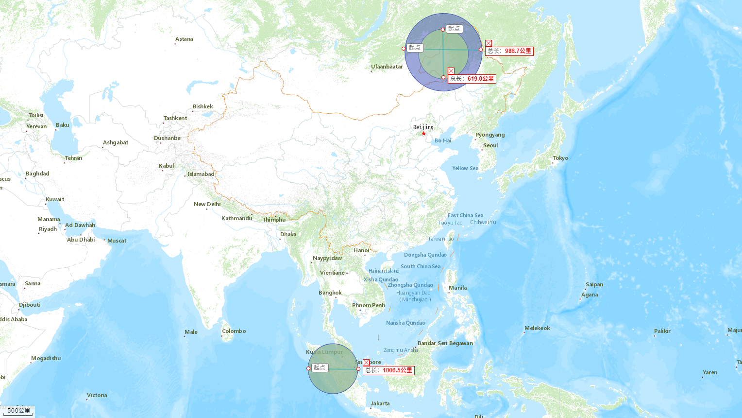
The green one is the non geographic buffer, and the blue one is the geographic buffer.
As we see the green one’s diameter is less than \(1000km\).
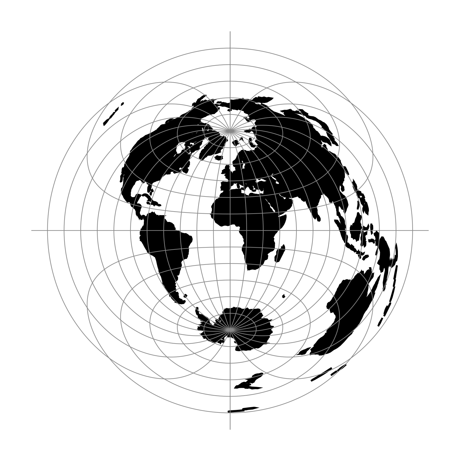
Problem of Non Geographic Buffer#
The following GIF could tell us why the green one is smaller than the blue one.
The EPSG:3857 is a cylindrical map projection, that cause the area which closes to the equator is the same as real.
Geographic Buffer#
Use Local Projection CRS#
A idea to fix this is to use local projection CRS. Local projection CRS means build projection CRS for each point.
The Steps to generate buffer would be following.
Transform each point of these geometries from default CRS to local projection CRS.
Transform them back to default CRS.
Do dissolve operation for generated buffers from geometry points.
In this way, it could totally describe the all points in Earth.
However, it would be so slow to get such great precision. And hard to vectorize this algorithm, because of different local projection CRS.
Use UTM CRS#
Another idea to fix this is to use Universal Transerse Mercator (UTM) projection CRS.
One projection would lose precision, much would slow down. The UTM CRS is a good balance between precision and speed.
It divides into sixty zones across the globe. The speed depends on the geometries where they are. It would be as quick as a normal speed if the zone of geometries is the same.
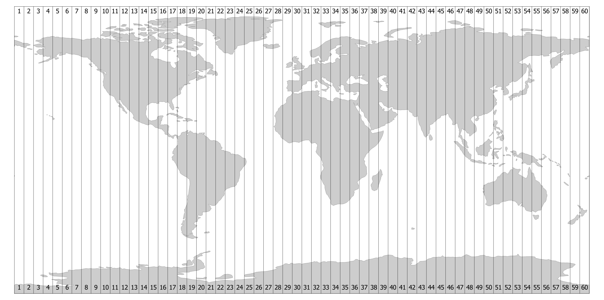
That is what the geobuffer() method does.
What’s next? Try to use it.